
|
D68 /
ApplicationToTheGarageScenarioThe above methodology will be applied to the garage scenario. In the HySafe internal project InsHyde releases in closed spaces have been studied. These studies were supported by experimental and numerical simulations of releases in garage-like geometries. In cooperation typical hydrogen sources were identified. So typical releases are in the order of 1 g H2/s. Assuming an orifice of 20 mm in diameter the gas velocity u at the exit would reach 38 m/s in average. 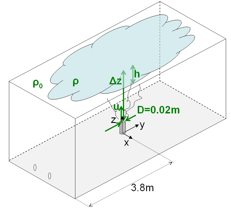 Figure 1. Setup of the garage scenario to be analysed The initial mixing tests in the INERIS gallery facility applied hydrogen directly. The INERIS facility is described in detail in the documents of the HySafe SBEP-V3 description http://www.hysafe.net/SBEPV3. The actual experiments are characterised by two time domains:
In the following chapter we will use the law approach to derive the relevant dimensionless quantities involved. The equation approach as explained in xyz? will be used to check the completeness (usually this step is not required). As the analysis of these dimensionless parameters will prove that perfect similarity may not be provided we will relax the problem by dividing the whole process in the two domains in the following sub-chapters. The initial vertical jet injection and the subsequent diffusion phase - as introduced above will be considered separately. For the first we will rely on models available from literature. For the latter we will apply a dimensional analysis. The release process when relatively light gases are injected at low Mach speed in the atmosphere is governed by the forces of inertia, buoyancy and viscosity. Hence the following laws apply: Law for interial forces $$ F_{inertia} \simeq \rho L^2 V^2 \Rightarrow \Pi_i = { F \over {\rho L^2 V^2}} $$ Law for gravitational forces $$ F_{gravitation} \simeq \Delta \rho L^3 g \Rightarrow \Pi_g = { F \over {\Delta \rho g L^3 }} $$ Law for viscous forces $$ \tau \simeq \mu { V \over L } \Rightarrow F_{viscous} \simeq \mu L V \Rightarrow \Pi_v = { F \over {\mu L V }} $$ As we don't have any external characteristic force F, only ratios of the above ratios will be of interest. In these ratios the fictional force F drops out and we get two well known \Pi-Numbers from the above three laws: The Reynolds number Re $$ Re = { \Pi_v \over \Pi_i } = { L V \over \nu } $$ and the Richardson number Ri $$ Ri = { \Pi_i \over \Pi_g } = { {\Delta \rho g L } \over \rho V^2 } $$ It is easy to see that the Richardson number is closely related to the Froude number Fr introduced in the Equation Approach description: $$ Ri = { {\Delta \rho} \over \rho } { 1 \over Fr^2 } = { 1 \over Fr^{\star} } $$ Where Fr^{\star} defines the densimetric Froude number |