
|
BRHS /
Other Types of Releases
Contributing Authors
SubsonicGaseous hydrogen releases through a hole or a conduct are produced as a result of a positive pressure difference between a container and its environment. The aperture is often modeled as a nozzle. Depending on the upstream pressure, a flow through a convergent nozzle to a lower downstream pressure can either be chocked (or sonic) or subsonic. The crossover pressure is a function of the ratio of the constant volume to the constant pressure specific heat, see Hanna and Strimaitis (HannaSR:1989). The flow resulting from a subsonic release is basically an expanded jet. The concentration profile of hydrogen in this expanded jet is inversely proportional to the distance to the nozzle along the axis of the jet. At a given distance from the nozzle, the concentration profile of hydrogen in air is distributed according to a Gaussian function centered on the axis. The following formula has been suggested by Chen and Rodi (ChenCJ:1980) for the axial concentration (v/v) decay of variable density subsonic jets:
Where C(x) is the concentration (vol) at location x, Cj is the concentration at the outlet nozzle, dj is the jet discharge diameter, ρα is the density of the ambient air, ρg the density of the gas at ambient conditions, x is the distance from the nozzle along the jet axis, x0 is the virtual absicca of the hyperbolic decrease (usually neglected because it is of the order of magnitude as the real diameter) and K is a constant equal to 5. For hydrogen, chocked releases occur when the upstream pressure is 1.9 times larger than downstream, otherwise the flow is subsonic. The flow rate of a chocked flow is only a function of the upstream pressure, whereas the flow rate of a subsonic release will depend on the difference between the upstream and downstream pressures. A release from a compressed gas storage system into the environment will therefore be chocked as long as the storage pressure remains larger than 1.89 bars. A chocked release of hydrogen undergoes a pressure and a temperature drop at the exit of the nozzle. The pressure will drop until the exit pressure reaches the value of the downstream pressure. At that point, the release becomes subsonic and the exit pressure remains constant at the downstream value. In the chocked regime, the gas velocity at the exit of the nozzle is exactly the sonic velocity of the gas. The flow rate can therefore be estimated from
where ρ is the density of hydrogen at the exit of the nozzle, calculated using the local value of the temperature and the pressure. The flow rate will also be affected by the shape of the aperture, friction and the length of the conduit between the reservoir and the release point. Because the exit density changes as a function of temperature and pressure, and because the sonic velocity is essentially proportional to the square root of the temperature, the flow rate will not remain constant but will vary as the upstream pressure drops (Fig. 1). Figure 1 shows the effect of using real gas hydrogen properties compared to ideal gas. It is well known that at high storage pressures real hydrogen gas densities are lower than ideal gas densities. Table 1 compares real versus ideal hydrogen densities at temperature 288 K and pressures 200 and 700 bar, (values taken from the (MarshallN:1976) ). For given storage volume the real gas assumption results in less stored hydrogen mass and consequently less released mass in an accidental situation. Table 1: Comparison between real and ideal gas properties
The effect of real gas properties has been taken into account in the 1983 Stockholm hydrogen accident simulations by Venetsanos et al.(VenetsanosAG:2003), where tables from Encyclopedie des gaz were used to obtain the hydrogen density. Real gas properties calculations based on the Beattie�Bridgeman equation of state were reported by Mohamed and Paraschivoiu (MohamedK:2005) , who modeled a hydrogen release from a high pressure chamber. Real gas properties using the Abel-Nobel equation of state were considered by Cheng et al.(ChengZ:2005) who performed hydrogen release and dispersion calculations for a hydrogen release from a 400 bar tank through a 6 mm PRD opening and found that the ideal gas law overestimates the hydrogen release rates by up to 35% during the first 25 seconds after the release. Based on these findings these authors recommended a real gas equation of state to be used for high pressure PRD releases. 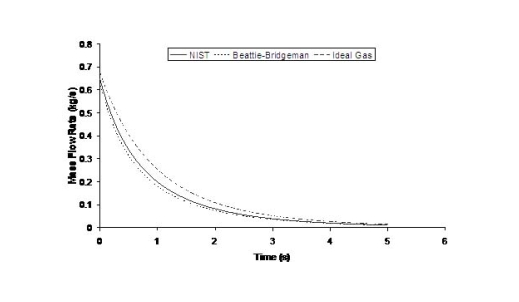 Fig. 1: Mass flow rate as a function of time from a 6 mm aperture of a 345 bar compressed gas 27.3 litre cylinder (calculated using the NIST (LemmonEW:2000) , the Bettie-Bridgeman and the ideal gas equations of state based on (MohamedK:2005). A chocked jet (Fig. 2) can be basically divided into an under-expanded region, where the flow becomes supersonic, forming a cone-like structure (the Mach cone) (Fig. 3); and an expanded region, which behaves similarly to an expanded subsonic jet. The under-expanded region is characterized by a complex shock wave pattern, involving bow and oblique shocks (Figs 3 and 4). 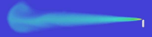 Fig. 2: Chocked release from a 150 litre 700 bar reservoir (AngersB:2006). 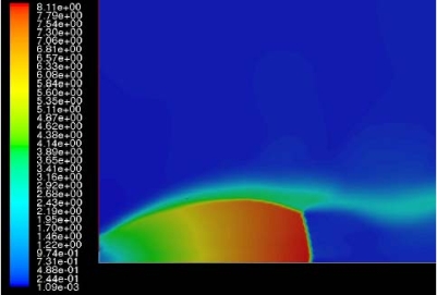 Fig. 3: Under-expanded chocked release of hydrogen (the Mach number is calculated with respect to air). 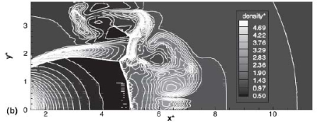 Fig. 4: Normalized density contours as a function of position (hydrogen jet in hydrogen atmosphere; source: (PedroG:2006) As for subsonic releases, the concentration profile of hydrogen in the expanded region is inversely proportional to the distance to the nozzle along the axis of the jet and is distributed according to a Gaussian function at a fixed distance from the nozzle. The axial concentration decay can be calculated using the formula for variable density subsonic jets, see Eq.(1), where the discharge diameter is replaced by the effective diameter, which is representatve of the jet diameter at the start of the subsonic region, i.e. after the Mach cone.
For the determination of the effective diameter various approaches have been proposed, such as (BirchAD:1984), (EwanBCR:1986) and (BirchAD:1987). In this latest approach, the effective diameter and corresponding effective velocity is calculated by applying the conservation of mass and momentum, between the outlet and a position beyond the Mach cone where pressure first becomes equal to the ambient, assuming no entrainment of ambient air.
Where ρj and uj are the density and the velocity of the jet at the outlet (respectively), ueff is the effective velocity, dj the diameter of the outlet. The effective velocity is calculated using the following expression:
where pj is the pressure of the jet at the outlet and pα is the ambient pressure. Regarding the constant K entering Eq.(3), different values have been reported in the literature. An average value of 4.9 is mentioned by Birch (BirchAD:1984) . An average value of 5.4 was reported in (BirchAD:1987) . This approach ((BirchAD:1984) and (BirchAD:1987) ; (HoufW:2005)) has been validated experimentally for vertical chocked releases for pressures below 70 bars for natural gas and hydrogen. A lower value K = 3.7 was reported by Ruffin (RuffinE:1996) who investigated experimentaly the concentration field of horizontal supercritical jets of methane and hydrogen for 40 bars storage pressure and with orifice diameters in the range from 25 to 150 mm. Ruffin et al. used the Birch approach (BirchAD:1984) in defining the effective diameter. Furthermore, Chaineaux (ChaineauxJ:2006) referring to the experiments in (ChaineauxJ:1999) reported a value of 2.25 for 200 bar hydrogen release from a 0.5 mm hole and a value of 2.89 for 700 bar hydrogen release from a 0.35 mm hole. Other experiments supporting the decay law of Eq.(3) are the experiments by Chitose et al. (ChitoseK:2006) who have measured the concentration profile of a hydrogen release from a 40 MPa storage unit. They observed that as a function of distance, the concentration profile of leaks with diameters ranging from 0.25 to 2 mm was inversely proportional to the distance to the nozzle and that all data points fell on a simple inverse power scaling law as a function of the normalized distance. Based on the experimental work, they obtained flammable concentration extents of 2.6 m, 6.6 m and 13.4 m for leak diameters of 0.2, 0.5 and 1.0 mm respectively. An experiment to measure the concentration profile of a horizontal release using a 10 mm diameter leak through a broken pipe from a 40 MPa storage unit showed that the extent of the 4% (vol) concentration envelope reached a distance of about 18 meters, 3 seconds after release. Flammable release extents can approximately be calculated using Eq.(3). The maximum extent of a time-dependent release will not be estimated using the initial storage pressure, but using a later value (see Houf and Schefer, (HoufW:2005)). Predicted flammable release extents are shown in Fig. 5 below. The axial distance to the lower flammability limit of 4% (vol) for hydrogen varies from 2 to 53 m for leak diameters ranging from 0.25 mm to 6.35 mm if the storage pressure is 1035 bars. 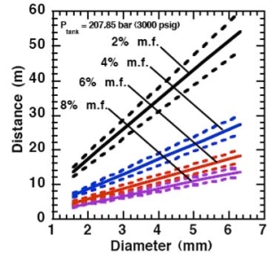 Fig. 5: Distances to concentrations of 2.0%, 4.0%, 6.0%, and 8.0% mole fraction on the centreline of a jet release from a 207.85 bars tank for various leak diameter obtained using the Sandia/Birch approach. The dashed lines indicate upper and lower bounds with �10% uncertainty in the value of the constant K. (from (HoufW:2007)) ReferencesLIST,NS Two phase jetsThe phenomena associated with two phase jet dispersion are reviewed by Bricard and Friedel (BricardP:1998). Within a short distance just downstream from the outlet, the flow can experience drastic changes which must be considered for subsequent dispersion calculations. The physical phenomena taking place in this region comprise (i) flashing if the liquid is sufficiently superheated, (ii) gas expansion when the flow is choked and (iii) liquid fragmentation. The corresponding quantities to be determined as initial conditions for subsequent dispersion calculations are the flash fraction, the jet mean temperature, velocity and diameter, and the droplet size. 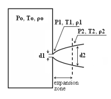 Fig. 1: Model of a two-phase flashing jet Flashing occurs when the liquid is sufficiently superheated at the outlet with respect to atmospheric conditions and corresponds to the violent boiling of the jet. The vapour mass fraction after flashing is most often determined in the models by assuming isenthalpic depressurization of the mixture between the outlet (position 1 in Fig. 1) and the plane downstream over which thermodynamic equilibrium at ambient pressure is attained (position 2 in Fig. 1):
Where Hfg is the latent heat of vaporization and Cpf is the liquid specific heat. When the flow is choked at the outlet, the gas phase expands to ambient pressure within a downstream distance of about two orifice diameters. This causes a strong acceleration of the two-phase mixture and usually an increase of the jet diameter. In the models, the velocity and diameter of the jet at the end of the expansion zone are given by the momentum and mass balance, respectively, integrated over a control volume extending from the outlet (position 1) to the plane where atmospheric pressure is first reached (position 2). It is assumed that no air is entrained in this region. The approach is similar to the one described above for choked gaseous hydrogen jets. The corresponding equations according to Fauske and Epstein (FauskeHK:1988) are:
Liquid fragmentation (or atomization) is caused by two main physical mechanisms: flashing and aerodynamic atomization. With flashing atomization, the fragmentation results from the violent boiling and bursting of bubbles in the superheated liquid, whereas aerodynamic atomization is the result of instabilities at the liquid surface. The determination of the initial droplet size (position 2) is a required initial condition, if the subsequent dispersion models account for fluiddynamic and thermodynamic non-equilibrium phenomena, like rainout and/or droplet evaporation. In the case of aerodynamic fragmentation, the maximum stable drop size is usually given by a critical Weber number, which represents the ratio of inertia over surface tension forces:
Where σ is the surface tension of the liquid, ρg is the gas density, dmax is maximum stable droplet diameter and ΔU the mean relative velocity between both phases. A range of values are used for the maximum Weber number, see (BricardP:1998) with 12 being the most common value. In the previous discussion the mass flow rate and outlet conditions (position 1) were assumed known. Hanna and Strimaitis (1989)(HannaSR:1989) have reviewed various approaches for calculating the release mass flow rate for liquid and two-phase flow releases. Detailed information on the subject can be found in chapter 15 of Lees (LeesFP:1996a) , in chapter 9 of Etchells and Wilday (EtchellsJ:1998) as well as in the older review of critical two phase flow models by D�Auria and Vigni (DAuriaF:1980) If the liquid in the reservoir is at saturated conditions, and if equilibrium flow conditions are established (i.e. for outflow pipe lengths > 0.1 m) then the two-phase choked mass flux (kg s-1 m-2) can be calculated following Fauske and Epstein (FauskeHK:1988):
Where Hfg is the latent heat of vaporization, Cpf is the liquid specific heat, T is the saturation temperature which is function of the storage pressure p, vg, vf are the saturated vapour and liquid specific volumes. This equation applies only if the vapor mass fraction after depressurization to atmospheric pressure (position 2) obeys the following criterion:
Figure 2 shows the equilibrium choked mass flux calculated using Eq. (4) for an LH2 release as function of the storage pressure. 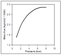 Fig. 2: Mass flux calculated using Eq. (4) for an LH2 release, as function of the storage pressure ReferencesInvalid BibTex Entry! Buoyant jets and plumesAfter the hydrogen-rich cloud losses its inertia, buoyant forces become more and more dominant. Usually, this cloud is less dense than the surrounding air and then the buoyancy force is directed upwards. When the hydrogen released is very cold, buoyant forces could point downwards. However, the heat and mass transfers during the mixing process reduce the mixture density and invert the buoyant force direction. The fluid structure established is a plume, where two regions are distinguished: forced plumes and buoyant plumes. At the forced plume both forces (inertia and buoyancy) are of similar magnitude and separate pure inertia region (jet) apart from the pure buoyant region (plume). The buoyancy to inertia ratio is expressed by the densimetric Froude number:
where U0, ρ0 and d0 are the fluid velocity, the fluid density and the diameter at the break point, respectively, g is the gravity acceleration and ρ∞ is the bulk density. Using this dimensionless number, (GebhartB:1988) recommend the following expressions (Tab. 1) for the three regions of a vertical upward structure. The x-direction is along the centreline of the structure, uc, ρc and cc the fluid velocity, the fluid density, and concentration at the centreline. Notice that velocity (u) and concentration (c) profiles at any transversal plane are expressed by Gaussian functions. When the structure shape is very different from an upward vertical one, these regions need to be established by numerical simulations. Table 1: Recommended expressions for the three regions of a vertical upward structure from (GebhartB:1988).
ReferencesInvalid BibTex Entry! LHLiquefied gases are characterized by a boiling point well below the ambient temperature. If released from a pressure vessel, the pressure relief from system to atmospheric pressure results in spontaneous (flash) vaporization of a certain fraction of the liquid. Depending on leak location and thermodynamic state of the cryogen (pressure expelling the cryogen through the leak is equal to the saturation vapour pressure), a two-phase flow will develop, significantly reducing the mass released. It is connected with the formation of aerosols, which vaporize in the air without touching the ground. Conditions and configuration of the source determine features of the evolving vapour cloud such as cloud composition, release height, initial plume distribution, time-dependent dimensions, or energy balance. The phenomena that may occur after a cryogen release into the environment are shown in Fig. 1.  Fig. 1: Physical phenomena occuring upon the release of a cryogenic liquid LH2 VaporizationThe release as a liquefied gas usually results in the accumulation and formation of a liquid pool on the ground, which expands, depending on the volume spilled and the release rate, radially away from the releasing point, and which also immediately starts to vaporize. The equilibrium state of the pool is determined by the heat input from the outside like from the ground, the ambient atmosphere (wind, insolation from the sun), and in case of a burning pool, radiation heat from the flame. The respective shares of heat input from outside into the pool are depending on the cryogen considered. Most dominant heat source is heat transport from the ground. This is particularly true for LH2, where a neglection of all other heat sources would result in an estimated error of 10-20%. For a burning pool, also the radiation heat from the flame provides a significant contribution. This is particularly true for a burning LNG pool due to its much larger emissivity resulting from soot formation (DienhartB:1995). Upon contact with the ground, the cryogen will in a short initial phase slide on a vapor cushion (film boiling) due to the large temperature difference between liquid and ground. The vaporization rate is comparatively low and if the ground is initially water, no ice will be formed. With increasing coverage of the surface, the difference in temperatures is decreasing until � at the Leidenfrost point � the vapour film collapses resulting in enhanced heat transfer via direct contact (nucleate boiling). On water, there is the chance of ice formation which, however, depending on the amount of mass released, will be hindered due to the violent boiling of the cryogen, particularly if the momentum with which the cryogen hits the water surface is large. Unlike lab-scale testing (confined), ice formation was not often observed in field trials (unconfined). The vaporization behaviour is principally different for liquid and solid grounds. On liquid grounds, the vaporization rate remains approximately constant due to natural convection processes initiated in the liquid resulting in an (almost) constant, large temperature difference between surface and cryogen indicating stable film boiling. On solid grounds, the vaporization rate decreases due to cooling of the ground. The heat flux into the pool can be approximated as being proportional to t-1/2. The vaporization time is significantly reduced, if moisture is present in the ground due to a change of the ice/water properties and the liberation of the solidification enthalpy during ice formation representing an additional heat source in the ground. LH2 Pool SpreadingAbove a certain amount of cryogen released, a pool on the ground is formed, whose diameter and thickness is increasing with time until reaching an equilibrium state. After termination of the release phase, the pool is decaying from its boundaries and breaking up in floe-like islands, when the thickness becomes lower than a certain minimum which is determined by the surface tension of the cryogen (in the range of 1 to 2 mm). The development of a hydraulic gradient results in a decreasing thickness towards the outside. The spreading of a cryogenic pool is influenced by the type of ground, solid or liquid, and by the release mode, instantaneous or continuous. In an instantaneous release, the release time is theoretically zero (or release rate is infinite), but practically short compared to the vaporization time. Spreading on a water surface penetrates the water to a certain degree, thus reducing the effective height responsible for the spreading and also requiring additional displacement energy at the leading edge of the pool below the water surface. The reduction factor is given by the density ratio of both liquids telling that only 7% of the LH2 will be below the water surface level compared to, e.g., more than 40% of LNG or even 81% of LN2. During the initial release phase, the surface area of the pool is growing, which implies an enhanced vaporization rate. Eventually a state is reached which is characterized by the incoming mass to equal the vaporized mass. This equilibrium state, however, does not necessarily mean a constant surface. For a solid ground, the cooling results in a decrease of the heat input which, for a constant spill rate, will lead to a gradually increasing pool size. In contrast, for a water surface, pool area and vaporization rate are maximal and remain principally constant as was concluded from lab-scale testing despite ice formation. A cutoff of the mass input finally results in a breakup of the pool from the central release point creating an inner pool front. The ring-shaped pool then recedes from both sides, although still in a forward movement, until it has completely died away. A special effect was identified for a continuous release particularly on a water surface. The equilibrium state is not being reached in a gradually increasing pool size. Just prior to reaching the equilibrium state, the pool is sometimes rather forming a detaching annular-shaped region, propagates outwards ahead of the main pool (BrandeisJ:1983). This phenomenon, for which there is hardly experimental evidence because of its short lifetime, can be explained by the fact that in the first seconds more of the high-momentum liquid is released than can vaporize from the actual pool surface; it becomes thicker like a shock wave at its leading edge while displacing the ground liquid. It results in a stretching of the pool behind the leading edge and thus a very small thickness, until the leading edge wavelet eventually separates. Realistically the ring pool will most likely soon break up in smaller single pools drifting away as has been often observed in release tests. Whether the ring pool indeed separates or only shortly enlarges the main pool radius, is depending on the cryogen properties of density and vaporization enthalpy and on the source rate. Also so-called rapid phase transitions (RPT) could be observed for a water surface RPTs are physical ("thermal") vapor explosions resulting from a spontaneous and violent phase change of the fragmented liquid gas at such a high rate that shock waves may be formed. Although the energy release is small compared with a chemical explosion, it was observed for LNG that RPT with observed overpressures of up to 5 kPa were able to cause some damage to test facilities. Experimental WorkMost experimental work with cryogenic liquefied gaseous fuels began in the 1970's concentrating mainly on LNG and LPG with the goal to investigate accidental spill scenarios during maritime transportation. A respective experimental program for liquid hydrogen was conducted on a much smaller scale, initially by those who considered and handled LH2 as a fuel for rockets and space ships. Main focus was on the combustion behavior of the LH2 and the atmospheric dispersion of the evolving vapor cloud after an LH2 spill. Only little work was concentrating on the cryogenic pool itself, whereby vaporization and spreading never were examined simultaneously. The NASA LH2 trials in 1980 (ChirivellaJE:1986) were initiated, when trying to analyze the scenario of a bursting of the 3000 m3 of LH2 containing storage tank at the Kennedy Space Center at Cape Canaveral and study the propagation of a large-scale hydrogen gas cloud in the open atmosphere. The spill experiments consisted of a series of seven trials, in five of which a volume of 5.7 m3 of LH2 was released near-ground within a time span of 35-85 s. Pool spreading on a "compacted sand" ground was not a major objective, therefore scanty data from test 6 only are available. From the thermocouples deployed at 1, 2, and 3 m distance from the spill point, only the inner two were found to have come into contact with the cold liquid, thus indicating a maximum pool radius not exceeding 3 m. In 1994, the first (and only up to now) spill tests with LH2, where pool spreading was investigated in further detail, were conducted in Germany. In four of these tests, the Research Center Juelich (FZJ) studied in more detail the pool behavior by measuring the LH2 pool radius in two directions as a function of time (DienhartB:1995). The release of LH2 was made both on a water surface and on a solid ground. Thermocouples were adjusted shortly above the surface of the ground serving as indicator for presence of the spreading cryogen. The two spill tests on water using a 3.5 m diameter swimming pool were performed over a time period of 62 s each at an estimated rate of 5 l/s of LH2, a value which is already corrected by the flash-vaporized fraction of at least 30%. After contact of the LH2 with the water surface, a closed pool was formed, clearly visible and hardly covered by the white cloud of condensed water vapor. The "equilibrium" pool radius did not remain constant, but moved forward and backward within the range of 0.4 to 0.6 m away from the center. This pulsation-like behavior, which was also observed by the NASA experimenters in their tests, is probably caused by the irregular efflux due to the violent bubbling of the liquid and release-induced turbulences. Single small floes of ice escaped the pool front and moved outwards. After cutting off the source, a massive ice layer was identified where the pool was boiling. In the two tests on a solid ground given by a 2 x 2 m2 aluminum sheet, the LH2 release rate was (corrected) 6 l/s over 62 s each. The pool front was also observed to pulsate showing a maximum radius in the range between 0.3 and 0.5 m. Pieces of the cryogenic pool were observed to move even beyond the edge of the sheet. Not always all thermocouples within the pool range had permanent contact to the cold liquid indicating non-symmetrical spreading or ice floes which passed the indicator. Computer ModellingParallel to all experimental work on cryogenic pool behavior, calculation models have been developed for simulation purposes. At the very beginning, purely empirical relationships were derived to correlate the spilled volume/mass with pool size and vaporization time. Such equations, however, were according to their nature strongly case-dependent. A more physical approach is given in mechanistic models, where the pool is assumed to be of cylindrical shape with initial conditions for height and diameter, and where the conservation equations for mass and energy are applied [e.g., (FayJA:1978) and (BriscoeF:1980). Gravitation is the driving force for the spreading of the pool transforming all potential energy into kinetic energy. Drawbacks of these models are given in that the calculation is terminated when the minimum thickness is reached, that only the leading edge of the pool is considered, and that a receding pool cannot be simulated. State-of-the-art modeling applies the so-called shallow-layer equations, a set of non-linear differential equations based on the conservation laws of mass and momentum, which allows the description of the transient behavior of the cryogenic pool and its vaporization. Several phases are being distinguished depending on the acting forces dominating the spreading:
During spreading, the pool passes all three phases, whereby its velocity is steadily decreasing. For cryogens, these models need to be modified with respect to the consideration of a continuously decreasing volume due to vaporization. Also film boiling has the effect of reducing sheer forces at the boundary layer. Based on these principles, the UKAEA code GASP (Gas Accumulation over Spreading Pools) has been created by Webber (WebberDM:1991) as a further development of the Brandeis model (BrandeisJ:1983) and (BrandeisJ:1983a). It was tested mainly against LNG and also slowly evaporating pools, but not for liquid hydrogen. Brewer also tried to establish a shallow-layer model to simulate LH2 pool spreading, however, was unsuccessful due to severe numerical instabilities except for two predictive calculations for LH2 aircraft accident scenarios with reasonable results (BrewerGD:1981). At FZJ, the state-of-the-art calculation model, LAUV, has been developed, which allows the description of the transient behavior of the cryogenic pool and its vaporization (DienhartB:1995). It addresses the relevant physical phenomena in both instantaneous and continuous (at a constant or transient rate) type releases onto either solid or liquid ground. A system of non-linear differential equations that allows for description of pool height and velocity as a function of time and location is given by the so-called "shallow-layer" equations based on the conservation of mass and momentum. Heat conduction from the ground is deemed the dominant heat source for vaporizing the cryogen, determined by solving the one-dimensional or optionally two-dimensional Fourier equation. Other heat fluxes are neglected. The friction force is chosen considering distinct contributions from laminar and from turbulent flux. Furthermore, the LAUV model includes the possibility to simulate moisture in a solid ground connected with a change of material properties when water turns to ice. For a water ground, LAUV contains, as an option, a finite-differences submodel to simulate ice layer formation and growth on the surface. Assumptions are a plane ice layer neglecting a convective flow in the water, the development of waves, and a pool acceleration due to buoyancy of the ice layer. The code was validated against cryogen (LNG, LH2) spill tests from the literature and against own experiments. LN2 release experiments were conducted on the KIWI test facility at the Research Center Juelich, which was used for a systematic study of phenomena during cryogenic pool spreading on a water surface. The leading edge of the LN2 pool is usually well reproduced. There is, however, a higher uncertainty with respect to the trailing edge whose precise identification was usually disturbed by waves developed on the water surface and the breakup of the pool into single ice islands when reaching a certain minimum thickness. The post-calculations of LH2 pool spreading during the BAM spill test series have also shown a good agreement between the computer simulations and the experimental data (see Fig. 2) (DienhartB:1995).  Fig. 2: Comparison of LH2 pool measurements with respective LAUV calculations for a continuous release over 62 s at 5 l/s on water (left) and at 6 l/s on an Al sheet (right) During the tests on water, the pool front appears at the beginning to have shortly propagated beyond the steady state presumably indicating the phenomenon of a (nearly) detaching pool ring typical for continuous releases. The radius was then calculated to slowly increase due to the gradual temperature decrease of the ice layer formed on the water surface. Equilibrium is reached approximately after 10 s into the test, until at time 62.9, i.e., about a second after termination of the spillage, the pool has completely vaporized. Despite the given uncertainties, the calculated curve for the maximum pool radius is still well within the measurement range. The ice layer thickness could not be measured during or after the test; according to the calculation, it has grown to 7 mm at the center with the longest contact to the cryogen. The spill tests on the aluminum ground (right-hand side) conducted with a somewhat higher release rate is also characterized by a steadily increasing pool radius. The fact that the attained pool size here is smaller than on the water surface is due to the rapid cooling of the ground leading soon to the nucleate boiling regime and enhanced vaporization, whereas in the case of water, a longer film boiling phase on the ice layer does not allow for a high heat flux into the pool. This effect was well reproduced by the LAUV calculation. ReferencesInvalid BibTex Entry! Other Types of ReleasesPermeation leaksPermeation leaks involve diffusive transport of hydrogen molecules through the surface material. This is significantly more pronounced in storage tanks that do not have metallic containment, high storage pressure, have a high surface area and long residence times and occurs over an extended period of time. According to (ScheferRW:2006), permeation of hydrogen through a metal involves adsorption and dissociation of molecular hydrogen to atomic hydrogen on the inner surface, followed by diffusion of atomic hydrogen through the metal and finally recombination to molecular hydrogen and desorption at the outer surface. Equations are provided for the permeation rate of hydrogen through several common metals. The results show the sensitivity of hydrogen flux to type of material, temperature and pressure. In automotive applications for tanks without metallic containment (commonly referred to as Types 3 and 4, draft regulations and standards include limits on the acceptable permeation rates, For non-metallic liner materials, the draft ECE regulations permit a maximum hydrogen permeation rate of 1.0Ncm3/hr per litre internal volume of the container for the settled pressure at 150C for a full container at start of life (GRPE, 2003), while an SAE standard, J2578 adopts 75Ncm3/min (75NmL/min) at 850C/ end of life and at nominal working pressure for a standard passenger vehicle (the SAE rate is independent of the size of the storage system). ISODIS15869.3 permits up 2.8Ncm3/hr per litre internal volume of the container based on similar conditions to the ECE draft. ReferencesInvalid BibTex Entry! |